
Breathe…Change Data Capture (CDC) doesn’t have to be stressful. Well maybe just a little bit, but at least there’s a way to minimize it. After some surprisingly straight-forward configuring, your data can be consistently synced across multiple systems, preserving quality and integrity.
CDC or the process of capturing the real-time changes happening in a database has become essential for the replication, restoring, analysis and quality of data, especially in modern architectures where the same source data feeds multiple environments.
A relational database optimized to handle atomic transactions involving CRUD (create, read, update, delete) operations does not support a high volume of complex analytical queries–they eat up resources. Nor does it bother with historical data changes; only the current state of the data is kept. This is why we need separate storage like a warehouse.
‘But we have the Write Ahead Logs‘, you say. Yes we do, but they live in the same database that can’t handle all our analytics needs. They are considered to be the best source for historical changes, though; we just need to capture them to use them.
CDC Methods
If you go the query-based approach, you won’t capture hard deletes (because the record doesn’t exist anymore) unless you add a tracking column that uses labels to keep track of all deletes, but eventually this creates performance issues as the tables grow.
Performance issues also creep up in large datasets if you use trigger functions to replicate all the changes in an audit table. This creates too many write operations. And they still need to be extracted somehow to be used or shared. In a modern application where events occur in high velocity, trigger-based capture just can’t keep up.
For real-time streaming, log-based CDC is the winner. It is considered the most reliable, fastest method with the lowest load on a database. And it ensures that a change is logged only once and in the right order. This method only reads the logs, but building the pipeline to deliver them in time can be complex.
If you’d like to know more about CDC methods, see this article or check out the Wikipedia page.
Contents
Our Set Up
We’ll explore Estuary’s Flow to handle our CDC needs for a few reasons including:
- Building our own CDC pipeline is way too complicated
- It uses the log-based approach
- It is highly automated: if your source has schema changes like data types or new columns, no problem; schema inference is an option
- It provides low latency streaming in real time to multiple targets
- It is less complicated to implement than other options
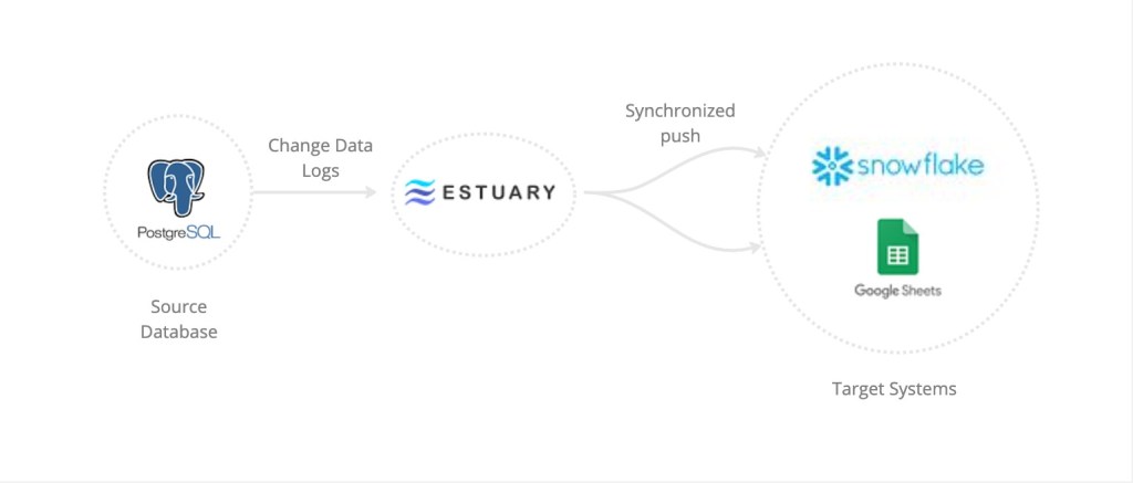
The source database will be PostgreSQL and we’ll use Snowflake for the target warehouse.
Also, we want to see the data synced across multiple targets, so we’ll include Google Sheets.
This allows for groups of users who have different skill sets to access the same data; a business analyst might prefer a user interface like spreadsheets over SQL queries.
Postgres & Flow
Connectors and Collections
To capture our change logs from Postgres, Flow provides a connector which is a plugin component that allows it to interface with endpoint data systems (by definition). It can also be used to load a target if it lives within Postgres. Estuary has many connectors for the most current needs and they are open-sourced.
Once we configure the connector, the captured logs will live in a collection (real-time data lake within Flow). One important feature is that changes to the collection are automatically synced in the downstream targets with a latency of milliseconds.
There is no need for a manual push or updating on our part, nor scheduling of running jobs like in other pipelines.
If you need to transform your capture data before it is saved in a collection, Flow offers derivations. By definition they are, in essence, a collection that is constructed from applying transformations to one or more sourced collections. They are updated automatically as changes are made to their source collections. They are currently supported in SQLite or TypeScript, with Python in the near future.
In this demo we don’t need to use derivations (perhaps that will be the followup article). But they have nice examples to explore in the documentation.
Postgres Hookup
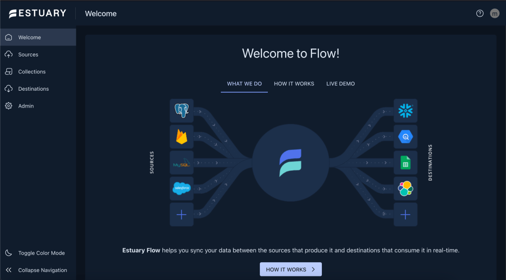
Flow has two environments for development: the web application and a CLI called flowctl to access their public API. We are going to use the web app since it’s very user friendly and better for demonstration purposes. Here is a view of the home page:
This connector works with self-hosted servers, AWS RDS and Aurora, Google Cloud SQL and Azure’s Database for PostgreSQL. In this demo we are following a self-hosted approach. More detailed set up docs here.
Before we configure the connector, we need to prep our database. Postgres Documentation
For PostgreSQL v14 you’ll need to run these commands:
CREATE USER flow_capture WITH PASSWORD 'secret' REPLICATION;
GRANT pg_read_all_data TO flow_capture;
Be sure to use a stronger password than 'secret'.
CREATE TABLE IF NOT EXISTS public.flow_watermarks (slot TEXT PRIMARY KEY, watermark TEXT);
GRANT ALL PRIVILEGES ON TABLE public.flow_watermarks TO flow_capture;
CREATE PUBLICATION flow_publication;
ALTER PUBLICATION flow_publication SET (publish_via_partition_root = true);
ALTER PUBLICATION flow_publication ADD TABLE public.flow_watermarks, <other_tables>;
Include the table(s) you intend to track in the last line for <other_tables>.
Next is the WAL (Write Ahead Log) level.
CALTER SYSTEM SET wal_level = logical;
Once this is run successfully, restart Postgres.
Next, you’ll need an internet-accessible address or set up SHH. To keep things simple, I used a tunnel to my local machine using ngrok, which reminds me…
Estuary has a nice support group through Slack. When I ran into an issue concerning this part of the hook up, they had my back with solutions. If you sign up for the free trial, you can join their #general channel for questions and updates.
Be sure to have your tunnel up and running before you fill out the config fields in the next section (if you choose to go that route).
To set up a connector: go to Sources from the right menu on the web app and click on ‘+ New Capture’, then choose the PostgreSQL option.
The endpoint configurations are simple:
- Server Adress: This is where you use the host:port generated for you by ngrok. It will look something like
2.tcp.ngrok.io:1832 - Database User to Authenticate:
flow_capture - Password for specified database user: use the password you created for flow_capture user in the commands above
- Database name to capture from: this is usually
postgres
Click ‘NEXT’ … if your connection data is set up correctly, you will advance to the next section, otherwise, you’ll get an error.
In the Target Collections section you’ll see the table name(s) you specified from which to capture the changes. In the Config section you have backfill options for each table. I chose to use ‘Only Changes’ for my purposes. See figure below:
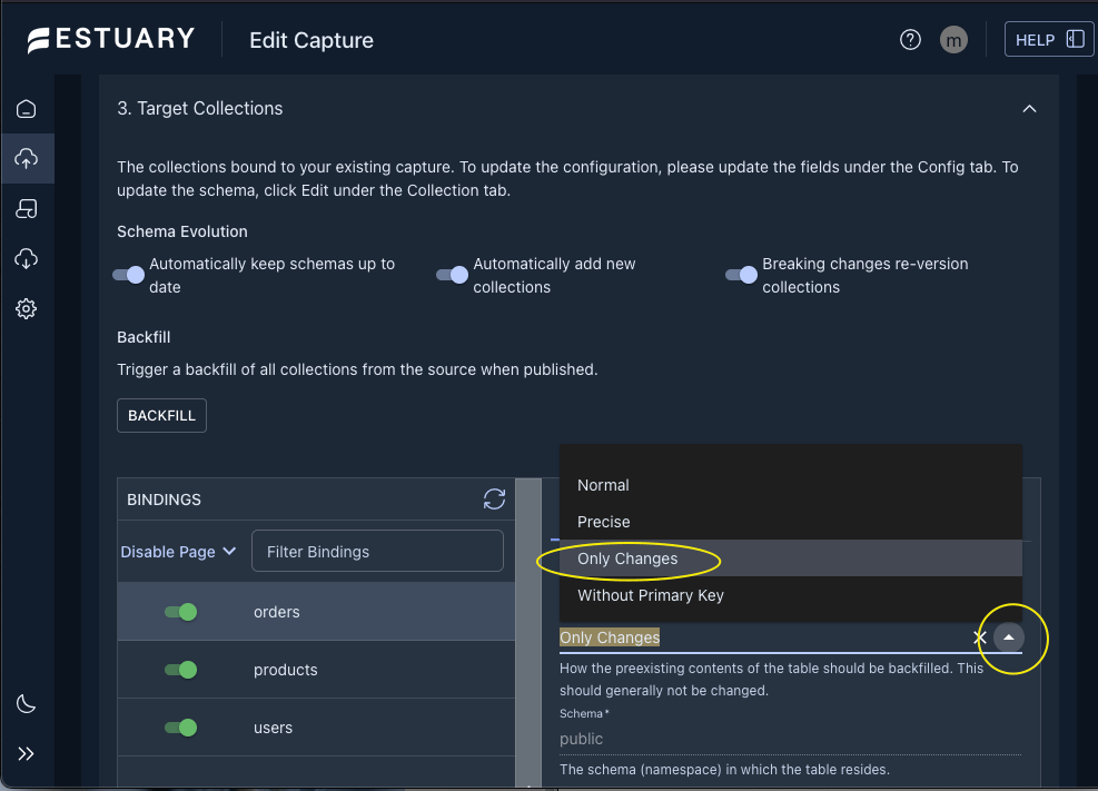
Also, I’d like to highlight the options available for schema changes right above the Backfill section. This is a nice feature as it takes away support tasks from my list!
I left the default settings since I want my collection to update the schema if anything is changed in my postgres database sometime.
Now you are ready to either ‘TEST’ or ‘SAVE AND PUBLISH’. If your test is good, then save and publish.
Your capture will show up in the Sources page and will start running automatically. A green dot next to it means it’s running, orange/yellow is pending, and red is stopped or some error occurred.
That’s it! We are now ready to hook up our targets.
Snowflake & Flow

Destinations
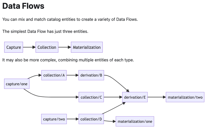
A destination in a Flow pipeline is called a materialization. You can set up this type of Flow task to bind one or more collections as its resources.
Now that we know the basic terminology we can consider the possible pipelines one can build as shown below.
Snowflake Hookup
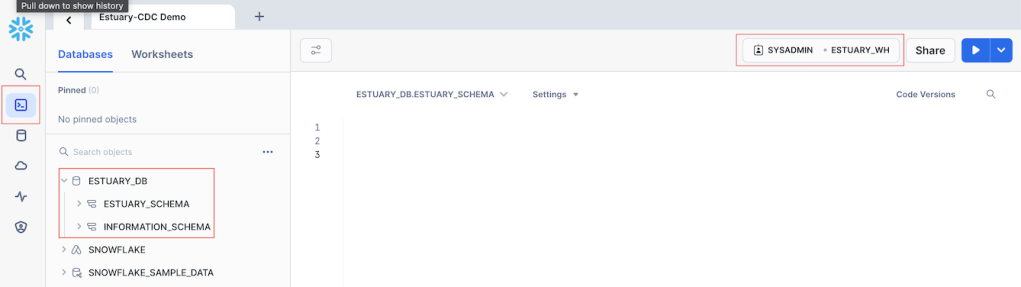
Some preliminary work is needed here. You’ll need a Snowflake account (30 day trial) where you set up a database and warehouse. I followed a portion of an example from Estuary’s docs here: documentation. Skip to the section ‘Prepare Snowflake to use with Flow‘ and follow the instructions in that section.
Your environment should look like this:
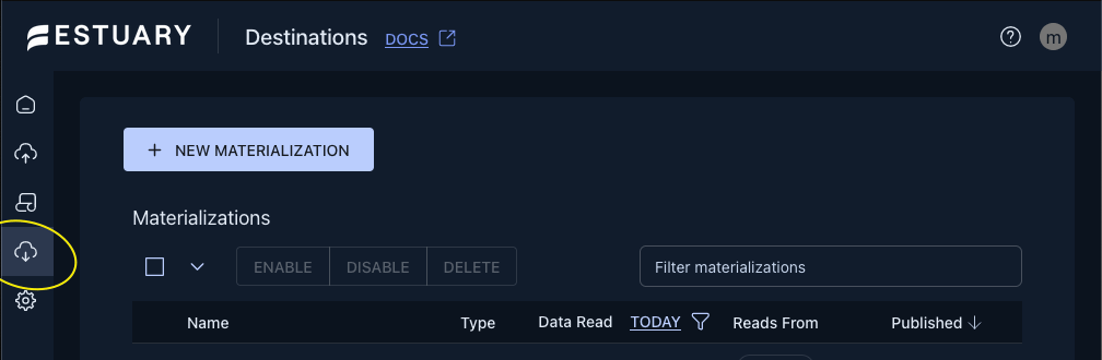
Next, in the web app click on ‘Destinations’ then ‘+ NEW MATERIALIZATION’ to find the connector for Snowflake.
To fill out the Details and Endpoint Config sections follow the steps in the ‘Materialize your Flow collection to Snowflake‘ section up to step 4 in the same example that we used above.
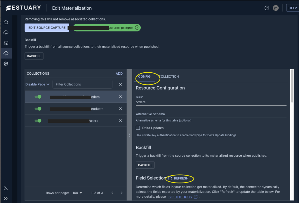
In the Source Collections section of your materialization editor choose the source capture that we created using postgres as a source. Once you do this, the collections list will be filled. In my case, I’m tracking three tables orders, products, and users.
This is the part we need to pick and choose which fields we want to push to Snowflake.
In the CONFIG tab scroll down to the REFRESH so that your fields are displayed for editing.
Now choose the Pointer option from the side menu option as seen below.
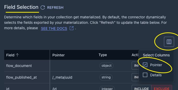
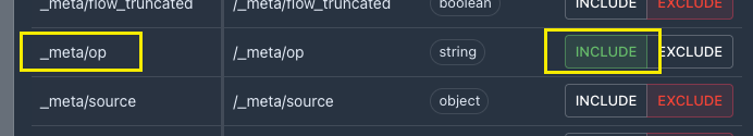
Now you should see a list of your familiar fields from the source table as well as some optional fields created by Flow for metadata.
You can explore with these as you like, but since we are particularly interested in CRUD operations from the WAL logs, we need to INCLUDE the /_meta/op field which will be populated by indicators for create/insert, update, and delete as ‘c’, ‘u’, ‘d’ respectively.
For our demo, this is all we need to do for each table we are tracking.
SAVE AND PUBLISH at this point. If all goes well your materialization will show up on the list of Destinations and will be automatically enabled.
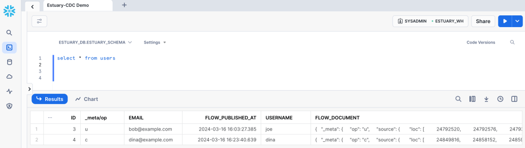
At this point you can test your pipeline to see if any changes in your postgres tables is captured and pushed to Snowflake. Just run either an UPDATE, INSERT, DELETE statement in a table and query the corresponding table in your new warehouse. I ran a few different ones in my users table. Notice the operation field which is handy for analysis!
Google Sheets Hookup
Our final destination is a spreadsheet from Google docs. This is the simplest connector so far and we’ll set it up in no time (almost).
Here are the instructions Estuary docs but it’s pretty straight forward when you start the materialization. All you need is an existing sheet, its URL, and authorization credentials. Be sure to choose the source collection from postgres that you created earlier.
You will have the same options to choose which fields to write on your sheet. Remember to include the /_meta/op field and any other that might interest you.
SAVE AND PUBLISH
Here you can see my destinations (I disabled them, but yours should be green).

Even if no changes are happening in your source database, the spreadsheet should be updated with a new tab for each table captured.
Capture Results
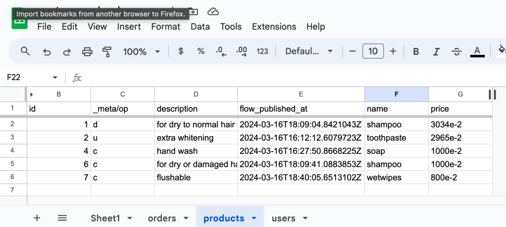
Finally you are ready to see any changes synced to both targets in real time (millisecond latency).
Repeat the steps you made to test the Snowflake target and compare the spreadsheet with your warehouse table(s). Notice the flow_published_at fields in both targets and how they are a match.

Conclusion
This simple pipeline can turn out to be a nightmare depending on the tools we choose to use. With Flow it was fairly painless to get this demo up and running; I think it took me longer to write about it. And we barely scratched the surface on what it can do. I am excited about pairing it up with a conversational app, since they offer a connector to the Pinecone vector database among others (I would appreciate my ever-changing knowledge base automatically synced with my vector store).
If you need to handle CDC for streaming data, Flow is a great solution. It removes the complexities of building your own pipelines from scratch, which might not be as fast in the end anyway. It is also easier to implement. But what I think is the most valuable feature is its ability to sync your data to all your destinations automatically.
If you’re curious about other approaches, check some comparisons here.

Leave a comment